Calculate JRO ISR Beam Location

For measurements made using a single beam, it may be more appropriate to account for the changes in beam direction with altitude when determining the measurement location instead of using the location of the radar. The method instruments.methods.jro.calc_measurement_loc() (see JRO) uses the beam azimuth and elevation measurements to determine the geodetic latitude and longitude.

This method is designed to be used with the JRO ISR data, and so assumes the azimuths and elevations have data variable names with the format 'eldir#' and 'azdir#' (where # is the beam number), or 'elm' and 'azm'. It will modify the pysat.Instrument.data object by adding latitude ('gdlat#') and longitude ('gdlon#') variables for every beam that has appropriately labeled azimuth and elevatiton data. If the azimuth and elevation angle variables don’t specify the beam number, # will be set to '_bm'.

The easiest way to use instruments.methods.jro.calc_measurement_loc() is to attach it to the JRO ISR pysat.Instrument as a custom function before loading data. If necessary, also download the desired data.

import datetime as dt
import pysat
import pysatMadrigal as pysat_mad

jro_obl = pysat.Instrument(inst_module=pysat_mad.instruments.jro_isr,
                           tag='oblique_long')
jro_obl.custom_attach(pysat_mad.instruments.methods.jro.calc_measurement_loc)

ftime = dt.datetime(2010, 4, 12)

if not ftime in jro_obl.files.files.index:
    jro_obl.download(start=ftime)

The geographic beam locations will be present alongside the azimuths and elevations after the data is loaded.

jro_obl.load(date=ftime)
'gdlat_bm' in jro_obl.variables and 'gdlon_bm' in jro_obl.variables

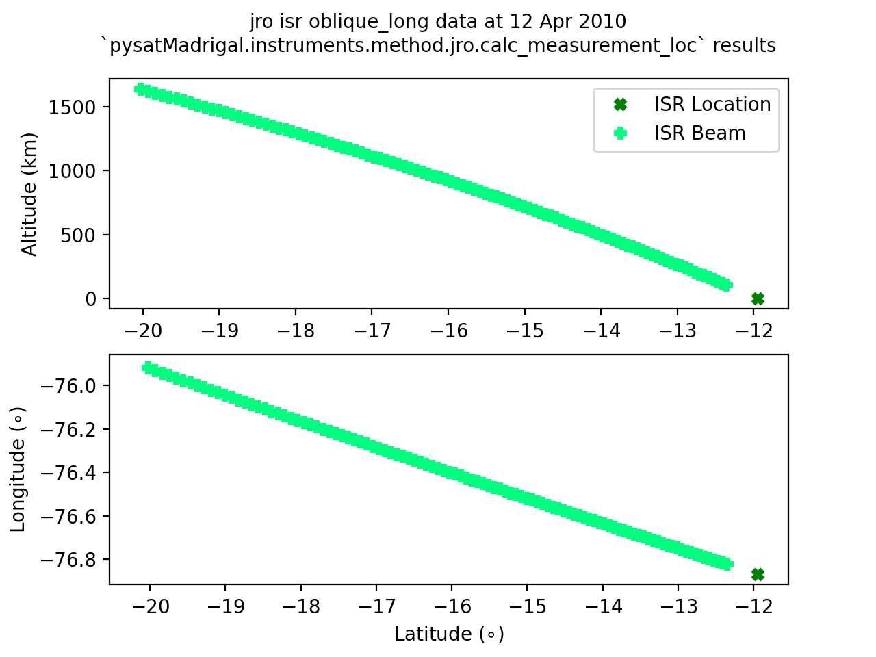
The result of the above command should be True. To better visualize the beam location calculation, let us plot the locations of the beam range gates and the radar location.

import matplotlib.pyplot as plt

# Initialize the figure and axes
fig = plt.figure()
ax_alt = fig.add_subplot(211)
ax_geo = fig.add_subplot(212)

# Plot the altitude data
ax_alt.plot(jro_obl['gdlatr'], 0.52, 'X', color='green')
ax_alt.plot(jro_obl['gdlat_bm'], jro_obl['gdalt'], 'P', color='springgreen')

# Plot the lat/lon data
ax_geo.plot(jro_obl['gdlatr'], jro_obl['gdlonr'], 'X', color='green')
ax_geo.plot(jro_obl['gdlat_bm'], jro_obl['gdlon_bm'], 'P',
            color='springgreen')

# Format the figure
ax_geo.set_xlabel('Latitude ($\circ$)')
ax_geo.set_ylabel('Longitude ($\circ$)')
ax_alt.set_ylabel('Altitude (km)')
ax_alt.legend(['ISR Location', 'ISR Beam'], fontsize='medium')
fig.suptitle('{:s} {:s} {:s} data at {:s}\n`pysatMadrigal.instruments.method.jro.calc_measurement_loc` results'.format(
    jro_obl.platform, jro_obl.name, jro_obl.tag,
    jro_obl.index[0].strftime('%d %b %Y')), fontsize='medium')